Finite Graphs and NetworkX

Add representation and analysis of graph networks to your Python toolkit

Aug 22, 2025

Many areas of practical data analysis and systems reasoning are grounded in the idea of using a finite graph to represent a problem. Not only does this provide a way to structure data, but the structure itself may suit analysis by a variety of techniques.

We’re going to keep the context very straightforward in order to build intuition over a few articles. The dusty old math texts can stay on their shelves for this one.

Finite Graph Terminology

Finite Graph: a finite collection of nodes and edges.

Node: an object in a graph that will have 0 or more edges connecting it to other nodes.

Edge: a line in the graph that connects two nodes. It is acceptable for the same node to be on both ends of a connection.

import networkx as nx
import matplotlib.pyplot as plt
import pandas as pd
import random
import typing

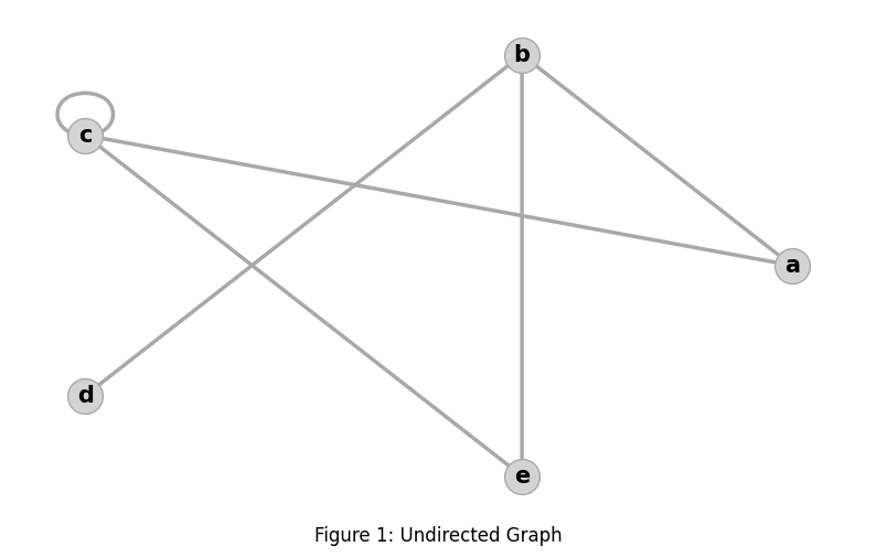
graph: nx.Graph = nx.Graph()
graph.add_nodes_from(['a', 'b', 'c', 'd', 'e'])
graph.add_edges_from([('a', 'b'), ('a', 'c'), ('b', 'd'),
                      ('c', 'c'), ('c', 'e'), ('e','b')])
node_positions: NodeLayout  = nx.circular_layout(graph)
nx.draw(graph, pos=node_positions, **draw_params())

Tuples like ('a', 'b') are the nodes at either end of that edge. As this is an undirected graph, ('b', 'a') would achieve the same.

The draw_params() function is a convenience for boilerplate reduction on setting rendering parameters across multiple examples.

def override_params(params: dict[str, typing.Any],
                    **kwargs: typing.Any) -> None:
    for key, value in kwargs.items():
        params[key] = value

def draw_params(**kwargs: typing.Any) -> dict[str, typing.Any]:
    params: dict[str, typing.Any] = dict(
        arrows=True,
        arrowsize=17,
        edge_color='darkgray',  # colors graph edges
        edgecolors='darkgray',  # colors border pixels of nodes
        font_color='black',
        font_size=15,
        font_weight='semibold',
        node_color='lightgray',
        node_size=525,
        width=2.5,
        with_labels=True,
    )
    override_params(params, **kwargs)
    return params

The complete code (available in a Jupyter notebook) renders:

Display of node labels is optional, which is a useful feature for large graphs. Just add with_labels=False to nx.draw() via the helper method draw_params():

nx.draw(graph, pos=node_positions, **draw_params(with_labels=False))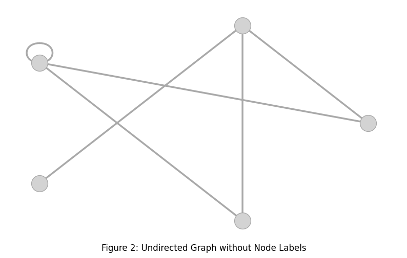

We can extend this idea a little further. We can give those edges a sense of direction.

Directed Finite Graph Terminology

Node: as defined previously.

Edge: a line in a graph that has a source node and a target node. When drawn, an arrow head points to the target node.

If the edges aren’t directed we call it an Undirected Finite Graph (or Undirected Graph for short), otherwise a Directed Finite Graph (again, Directed Graph for short).

Nodes in a directed graph now gain a bit more structure:

Outgoing Edges: the directed edges connected to a node that have that node as a source. Also called “outedges” in some math texts.
Incoming Edges: the directed edges connected to a node that have that node as a target. Also called “inedges” in some math texts.

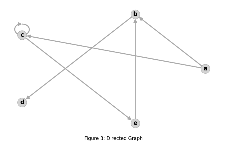
Representing edges is no different, except now the order of the identifier pairs matters when it didn’t matter for undirected edges. The first member of a pair is the source, the second is the target. The only substantial difference is the change in the NetworkX class used when defining the graph. We change the class from nx.Graph to nx.DiGraph:

graph: nx.Graph = nx.DiGraph()
graph.add_nodes_from(['a', 'b', 'c', 'd', 'e'])
graph.add_edges_from([('a', 'b'), ('a', 'c'), ('b', 'd'),
                      ('c', 'c'), ('c', 'e'), ('e','b')])
node_positions: NodeLayout  = nx.circular_layout(graph)
nx.draw(graph, pos=node_positions, **draw_params())

With this change the rendering becomes:

Alternate Representations

It can be mathematically useful, particularly for directed graphs, to think of them as corresponding to a matrix. Each row of a matrix corresponds to a source node, and each column corresponds to a target node. This is referred to as an Adjacency Matrix.

adj_rows: dict[typing.Hashable, list[typing.Any]] = dict(
    a=[0, 1, 1, 0, 0],
    b=[0, 0, 0, 1, 0],
    c=[0, 0, 1, 0, 1],
    d=[0, 0, 0, 0, 0],
    e=[0, 1, 0, 0, 0]
)
adj_matrix = pd.DataFrame.from_dict(adj_rows,
                                    orient='index',
                                    dtype=int,
                                    columns=list(adj_rows.keys()))
graph = nx.from_pandas_adjacency(adj_matrix, create_using=nx.DiGraph)
node_positions: NodeLayout  = nx.circular_layout(graph)
nx.draw(graph, pos=node_positions, **draw_params())

We use the Pandas trick of providing a keyed dictionary for rows and specifying the orientation. Thinking in terms of a known source having various targets is more intuitive than what column-specified data would force on us: to think in terms of one target having multiple sources. It also allows the visual aid of the text for populating adj_rows to correspond to how we have been taught to conceive of matrices. All we need to do is inform Pandas what the column keys are, which in this case is the same as the row keys: columns=list(adj_rows.keys()).

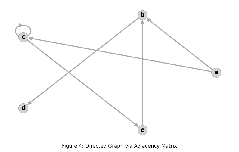
The output is the same as before, which was the goal. This representation can be convenient when the existing understanding of a graph is organized in terms of outgoing edges, because all the outgoing edge connections for a node form the matrix row for that node.

The number 1 in the matrix indicates a directed edge from the source (the row index) to the target (the column index). Using 0 and 1 is a traditional starting point for adjacency matrices because it supports some useful linear algebra, but there is no constraint that only the number 1 be used to indicate a connection. Any non-zero value can represent, for example, weight or length.

The disadvantage of this representation, at least with NetworkX, is that the only information this can capture are node names, edge directions, and a single edge weight. Adjacency matrices for NetworkX do not support the idea of structured objects so we couldn’t use one to specify multiple per-edge attributes. For that we need Edge Lists.

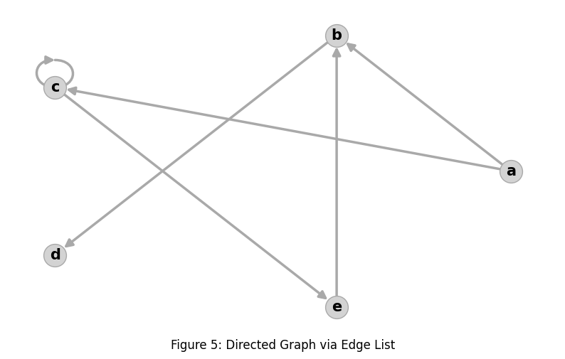
edge_rows = [
    dict(src='a', dest='b'),
    dict(src='a', dest='c'),
    dict(src='b', dest='d'),
    dict(src='c', dest='c'),
    dict(src='c', dest='e'),
    dict(src='e', dest='b'),
]
edge_list_df: pd.DataFrame = pd.DataFrame(edge_rows)
graph = nx.from_pandas_edgelist(edge_list_df,
                                source='src',
                                target='dest',
                                create_using=nx.DiGraph)
node_positions: NodeLayout  = nx.circular_layout(graph)
nx.draw(graph, pos=node_positions, **draw_params())

The situation has changed a bit:

Each edge must be specified as a dictionary with consistent keys indicating the source and target of the edge.
The edge list is converted into a Pandas DataFrame, and the dictionary keys become the column names.
We use nx.from_pandas_edgelist() to convert the DataFrame into a graph, which requires specifying the keys that were used for the source and target.

The final rendering though, at least for this data, is unchanged:

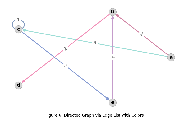
Now we can push this further to add more attributes to the edge data:

def random_color_channel() -> float:
    if not hasattr(random_color_channel, 'rand'):
        random_color_channel.rand = random.Random(42)
    return random_color_channel.rand.uniform(0.5, 1)

def random_rgb_color() -> tuple[float, float, float]:
    return random_color_channel(),
           random_color_channel(),
           random_color_channel()

edge_rows = [
    dict(src='a', dest='b', weight=1, color=random_rgb_color()),
    dict(src='a', dest='c', weight=3, color=random_rgb_color()),
    dict(src='b', dest='d', weight=2, color=random_rgb_color()),
    dict(src='c', dest='c', weight=1, color=random_rgb_color()),
    dict(src='c', dest='e', weight=2, color=random_rgb_color()),
    dict(src='e', dest='b', weight=1, color=random_rgb_color()),
]
edge_list_df: pd.DataFrame = pd.DataFrame(edge_rows)
graph = nx.from_pandas_edgelist(edge_list_df,
                                source='src',
                                target='dest',
                                edge_attr=['weight', 'color'],
                                create_using=nx.DiGraph)
edge_weights = nx.get_edge_attributes(graph, 'weight')
edge_colors = nx.get_edge_attributes(graph, 'color').values()
node_positions: NodeLayout  = nx.circular_layout(graph)
nx.draw(graph, pos=node_positions, **draw_params(edge_color=edge_colors))
nx.draw_networkx_edge_labels(graph, pos=node_positions,
                             **edge_label_params(edge_labels=edge_weights))

Now we’re adding some complexity:

Edges have two attributes: weight and color.
The color is an RGB triple where each channel is a float in the range [0, 1].
When using nx.from_pandas_edgelist() to produce a graph we have to tell it about the per-edge attributes: edge_attr=['weight', 'color']
NetworkX doesn’t do much with complex edges so we have to extract the data as edge_weights and edge_colors to use later as parameters.
The nx.draw() function has limited smarts on some forms of rendering, so we include use of nx.draw_networkx_edge_labels() to render the weights as values on each edge.
The way nx.draw() and nx.draw_networkx_edge_labels() share an understanding of node locations is via the node_positions layout object. In the previous examples it was only used once per rendering so its role was less apparent, but here we see it used to layer on rendering details. The object provides node coordinates in the rendering. I added a Python type alias to cover the kinds of data passed back by various layout algorithms:

NodeLayout: typing.TypeAlias = dict[typing.Hashable, list[float]]

Now we get a much richer rendering with per-edge weight labels and per-edge colors:

In future articles I expect to need to use various analytic techniques on graphs. Even without that, NetworkX can help with rendering images that support an explanation for how data is being transformed or analyzed.

References

Edits

2025-08-22: Added terminology for inedges and outedges.