Markov Chains with NetworkX and PyDTMC

An easy introduction to Markov Chains in Python

Aug 25, 2025

The brief segue into finite graphs in the previous article has paved the way for developing a little intuition on Markov Chains and working with them in Python. We will want this material for future data engineering explorations.

The concept of a Markov Chain is easy enough:

You have a collection of states.
There are probabilities of transitioning from the current state to various future states.
There is no memory behind those probabilities; if you know the current state then you know the probabilities of transitioning next to other states.

Prev: Finite Graphs and NetworkX | Next: Markov Chain Convergence in Python

We’re going to simplify the variety of Markov Chains we’ll be working with.

We will only discuss chains with a finite number of states.
Transitions from one state to the next happen in discrete time steps, not over the flow of continuous time. This lets us organize discussions in terms of time steps t0, t1, …

With those clarifications, what we’ll have are Discrete-Time Finite Markov Chains.

The use of the word ‘chain’ is intended to communicate that we can keep repeating this process of random state transitions over and over again. That assumes there are no states without any outgoing transitions, which are called absorbing states, which can terminate some randomly-generated walks.

The Graph Connection

Remembering our previous discussion on graphs, a Directed Finite Graph has:

Nodes.
Edges between pairs of nodes, and those edges are ordered from source to target.
When an edge leaves a source node, that is an outedge.
When an edge arrives (the arrow-head in a picture points at) a target node, that is an inedge.
It is something useful to assign attributes like a numeric weight to edges.

We’ll add to this a little bit of simplified statistical terminology.

A probability is a real number p where 0 ≤ p ≤ 1.
A discrete probability distribution is a finite collection of probability values that add up to 1.
If we have estimated or assigned probabilities to a collection of possible events, and those probabilities form a probability distribution, we refer to that collection of events as being stochastic.

And now we’re ready to characterize our Discrete-Time Finite Markov Chains (DTFMCs to save typing) in terms of Directed Finite Graphs (DFGs).

States in a DTFMC are nodes in a DFG.
If it is possible to transition between two states a and b in a DTFMC, then that is represented as the edge (a, b) in a DFG.
The probability of such a transition from state a to state b in a DTFMC is represented as the weight of the edge (a, b).
In an adjacency matrix for the DFG, each row corresponds to a source state and each column corresponds to a target state. All non-zero values will be the weights (probabilities of a possible state-to-state transition).
For every node (state) in the DFG, its collection of weighted outedges (representing state transitions with non-zero probability) is stochastic.

That last two points tell us that when the DFG for a DTFMC is represented as an adjacency matrix, each row will either sum to:

0 if and only if that state has no outedges.
1 if and only if that state has at least 1 outedge.

This representation of a Markov Chain is sometimes referred to as row-stochastic or row-normalized. It would be possible to construct a matrix that instead was column-stochastic or column-normalized; in that case we would be seeing the probability distribution for how possible source states could transition to a target state. Row-stochastic is for understanding how a specific source leads to many potential targets, Column-stochastic is for understanding how many potential sources lead to a specific target. In this article we’ll be working with row-stochastic representations.

NetworkX Example

Consider the following taxi trip model as a Markov Chain:

States are destinations.
Edges are trips between destinations.
Weight probabilities are the odds of going from one destination to another.

Our specific data will be

From the airport, 70% of trips go to the hotel, 20% the hospital, 10% the mall.
From the hospital, 60% of trips go to the hotel, 40% the airport.
From the hotel, 40% of trips go to the mall, 40% the airport, 20% the hospital.
From the mall, 70% of trips go to the hotel, 20% the airport, 10% the hospital.

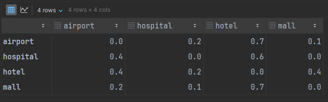
As shown in the previous article, we can represent such a weighted DFG as an adjacency matrix:

adj_rows = dict(
    airport= [  0, 0.2, 0.7, 0.1],
    hospital=[0.4,   0, 0.6,   0],
    hotel=   [0.4, 0.2,   0, 0.4],
    mall=    [0.2, 0.1, 0.7,   0],
)
adj_matrix = pd.DataFrame.from_dict(adj_rows,
                                    orient='index',
                                    dtype=float,
                                    columns=list(adj_rows.keys()))
graph = nx.from_pandas_adjacency(adj_matrix, create_using=nx.DiGraph)

We can use NetworkX to describe the appearance of the graph. First we describe the nodes and node labels:

node_colors = dict(
    airport='purple',
    hospital='red',
    hotel='blue',
    mall='darkgreen',
)

for node_name, node_color in node_colors.items():
    nx.draw_networkx_nodes(graph,
                           pos=node_positions,
                           nodelist=[node_name],
                           node_color=node_color,
                           **node_params())
label_colors = {node_name: node_name for node_name in node_colors}
nx.draw_networkx_labels(graph,
                        pos=node_positions,
                        labels=label_colors,
                        **node_label_params())

Then we describe the edges and edge labels:

for node in graph:
    out_edges_view = typing.cast(nx.reportviews.OutEdgeView, graph.out_edges)
    nx.draw_networkx_edges(graph,
                           pos=node_positions,
                           edgelist=out_edges_view(node),
                           edge_color=node_colors[node],
                           **edge_params())
    for src, target, data in out_edges_view(node, data=True):
        edge_label = {(src, target): data['weight']}
        nx.draw_networkx_edge_labels(graph,
                                     pos=node_positions,
                                     edge_labels=edge_label,
                                     font_color=node_colors[node],
                                     **edge_label_params())

This renders as:

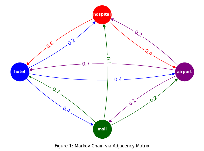
The outedges of each node are colored to match their source. The weights of all edges of the same color will add up to 1, reflecting their stochastic nature.

Now we have a visualization of a Markov Chain. From any state (node), in one discrete time step travel will happen on one of the correspondingly-colored outedges to a target node, with probability of that event as shown by the weight on the edge.

Counting DFG Walks

Going back for a moment to our graphs, we will introduce an additional concept.

A walk is a sequence of connected edges in a graph.
If the graph is a directed graph, edges only connect if each intermediate node functions first as a target for an edge, and then as a source for the next edge. Connections must respect directionality. If a graph has a directed edge (a, b), and another edge (c, b), you cannot directly connect those edges in a walk because they are going in opposite directions.

Given a particular DFG, between any two nodes, how many walks can we identify of length 2? Length 3? The answer is given by raising the unweighted adjacency matrix to the corresponding power. In other words if A is the adjacency matrix of a DFG, then the matrix product A * A computes the number of paths of length 2, and so on.

This can be illustrated with NetworkX and an edge list for weather transitions:

edge_rows = [
    dict(src='cloud', dest='cloud'),
    dict(src='cloud', dest='hail'),
    dict(src='cloud', dest='rain'),
    dict(src='cloud', dest='snow'),
    dict(src='cloud', dest='sun'),
    dict(src='hail', dest='cloud'),
    dict(src='hail', dest='hail'),
    dict(src='hail', dest='rain'),
    dict(src='rain', dest='cloud'),
    dict(src='rain', dest='hail'),
    dict(src='rain', dest='rain'),
    dict(src='rain', dest='snow'),
    dict(src='snow', dest='cloud'),
    dict(src='snow', dest='rain'),
    dict(src='snow', dest='snow'),
    dict(src='sun', dest='cloud'),
    dict(src='sun', dest='sun'),
]
edge_list_df = pd.DataFrame(edge_rows)
graph = nx.from_pandas_edgelist(edge_list_df,
                                source='src',
                                target='dest',
                                create_using=nx.DiGraph)
adj_matrix = nx.to_pandas_adjacency(graph, dtype=int)
adj_matrix

The last step converted the edge list to an adjacency matrix as a Pandas DataFrame:

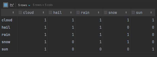
This data restricts sun to not spontaneously transitioning to hail or snow or rain. We would need a walk of length at least 2 to have a chance to transition through cloudy weather first. We can accomplish that with matrix multiplication as a “dot” product:

adj_matrix @ adj_matrix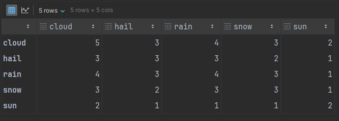

We can see, correctly, that there is only 1 walk of length 2 that starts with sun and ends with snow.

Also correct is the number of ways to start with sun and end with cloudy weather. There are 2: sun → sun → cloud and sun → cloud → cloud.

We don’t need to work with the adjacency matrix and figure out how many dot products to type in for higher powers. NetworkX provides a function to specify the desired power directly. It returns a dict of dicts, which we can make prettier as a Pandas DataFrame:

pd.DataFrame(nx.number_of_walks(graph, 2))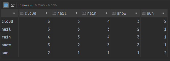

The results are the same as the calculation on the adjacency matrix.

The rest of the discussion will now return to exploring the taxi data.

Measuring DTFMC Walk Probabilities

In the DFG walk computations just shown, the weights in the adjacency matrix were all 1 to denote the directed edge. However, this same computation also works when the weights are other numbers, like probabilities. What is computed is the probability-weighted sum of those walks. This means:

Compute the n’th power of a Markov Chain.
We will get the probability of starting in a particular state a, and ending up in another state b. If there is no way to get from a to b then the value is 0.
This is the probability to have that outcome after exactly n steps in the walk.
The probability does not count the possibility of getting from a to b in fewer or greater than n steps.

Let’s try this for the taxi DTFMC defined earlier. The Pandas DataFrame for that adjacency matrix is:

We can compute the 3rd power of that graph. We’ll need to use the Pandas dot product for this, as NetworkX doesn’t understand weighting.

(adj_matrix @ adj_matrix) @ adj_matrix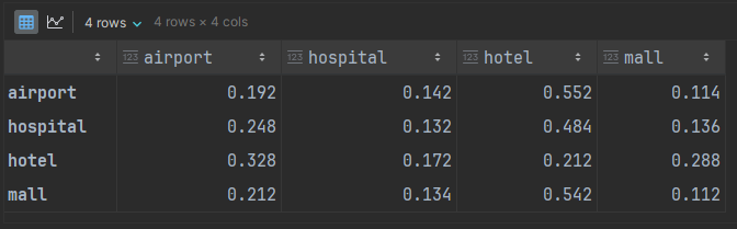

As we can see, starting at the mall and returning again on the third trip has an 11.2% probability. Also note that no entries are zero. We’ll discuss the implications shortly.

Markov Chains and PyDTMC

So far we’ve just been exploring how to represent a Markov Chain as a graph with an associated matrix with per-state probability distributions. We can do more to analyze the characteristics of the model of taxi data that we’ve built.

import pydtmc as mc

model = mc.MarkovChain(adj_matrix)
print(model)

From this we can get a summary report about our model:

DISCRETE-TIME MARKOV CHAIN
 SIZE:           4
 RANK:           4
 CLASSES:        1
  > RECURRENT:   1
  > TRANSIENT:   0
 ERGODIC:        YES
  > APERIODIC:   YES
  > IRREDUCIBLE: YES
 ABSORBING:      NO
 MONOTONE:       NO
 REGULAR:        YES
 REVERSIBLE:     NO
 SYMMETRIC:      NO

The important characteristics for now are that the model is:

Regular. This is a particularly strong property for a Markov Model to possess, and makes other operations much more approachable. It means that there is a probability distribution of states that all future state transitions will converge to.
Ergodic. All the states are reachable from each other after a finite number of steps (irreducible), and the long-term distribution of states does not oscillate with periodicity (aperiodic). Above there was a place where it was pointed out that the adjacency matrix raised to the third power had all positive entries: that showed the matrix was recurrent.
Recurrent: With a single recurrent class (meaning all states are in that class), we have that no matter which state we start in, we will return to it infinitely many times as we traverse more and more time steps.

Regular implies Ergodic, but the reverse is not always true.

Because we are dealing with Finite Markov Models, Recurrent implies Irreducible, and Irreducible implies Recurrent. These relationships would not hold for infinite models.

We can use PyDTMC to get that stationary distribution.

model.stationary_distributions

This is the probability distribution for visiting the states over time. The order of the states here is the same as the order of the rows in the original adjacency matrix, thus we spend the most time at the hotel: 0.4028777.

[array([0.25899281, 0.15107914, 0.4028777 , 0.18705036])]

We can obtain some insight into whether the model finds it easy or difficult to converge to that distribution. One way is by plotting the eigenvalues of the matrix:

mc.plot_eigenvalues(model)

From that we get:

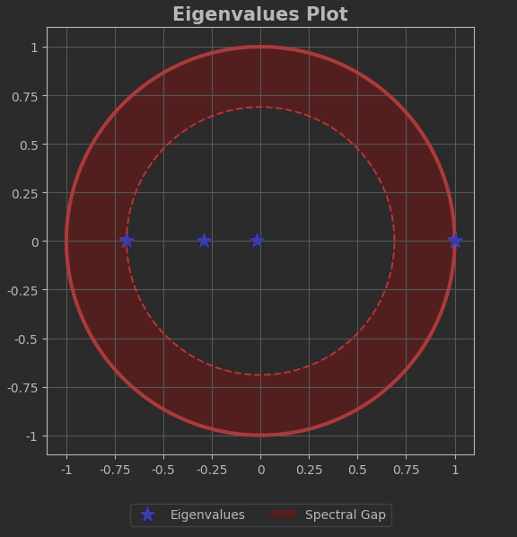
Take notice of the two largest-magnitude eigenvalues. The wide red ring shows the distance between them, called the spectral gap. The closer they are, the more difficult it is for the future probabilities to generate walk that converge to the stationary distribution.

We can find out the spectral gap directly:

model.spectral_gap

When the value is closer to 1, convergence is faster.
When it is closer to 0, convergence is slower.

0.31078141211367716

In our case convergence is a little sluggish.

We can get further insight into convergence with Spectral Density.

model.density

This tells us how variable the data is:

0.9166666666666666

A value near 1 suggests convergence is easier.
Near 0 indicates convergence is harder, and it would still mean that no matter what the spectral gap may be suggesting.

While it may sound a little counter-intuitive, data that is more variable actually makes convergence easier. When it is less variable then you have some low-probability transitions in the matrix that can keep the model stuck instead of moving freely around all its states.

In the next article we’ll explore what that convergence behavior looks like.

References

The Experimentalist : Markov Chains with NetworkX and PyDTMC © 2025 by Reid M. Pinchback is licensed under CC BY-SA 4.0