Markov Chain Convergence in Python

When does a Markov Chain ‘forget’ its starting point?

Aug 28, 2025

There are two direct benefits to training a Markov Chain on data. You can:

Analyze the structure of the model to understand the qualities of the data.
Generate new data that is very similar to the training data.

The focus of this article series is more the second point, but the first can help with the second. Trying to generate data raises some questions.

How do you know if the data generated actually is a reasonable facsimile of the training data?
Are there any inputs to the process, other than the training data, that could influence whether that generated data is a reasonable facsimile?
Much like with sampling in the field of statistics, how do you know when you have enough data from a Markov Chain?

Prev: Markov Chains with NetworkX and PyDTMC

Generating data from a Markov Chain requires an initial state to begin the process, and a random number each time we take a step. To cover these questions we will:

Create runs of output data. These are sequences of states.
Analyze the probability distribution of the states in those runs.
Make analysis repeatable by controlling random numbers via seeds.
Examine sensitivity of the runs to the choice of seed used.
Use all the possible initial states as initial states.
Assess how long it takes the model to “forget” the state it started with when generating output. We want it to forget because the choice of initial state is somewhat — later we’ll get into why I said “somewhat” — arbitrary, and we don’t want to wire a persistent bias into the generated data.

Some of this can be examined empirically by doing data-generation experiments and analyzing the results. Some can be estimated analytically via known techniques for Markov Chains.

We’ll be doing both. The empirical can help explain the purpose of the analytical.

Taxi Trips as a DTFMC, Revisited

Once again, here is our adjacency matrix that we use to build a Discrete-Time Finite Markov Chain.

adj_rows = dict(
    airport= [  0, 0.2, 0.7, 0.1],
    hospital=[0.4,   0, 0.6,   0],
    hotel=   [0.4, 0.2,   0, 0.4],
    mall=    [0.2, 0.1, 0.7,   0],
)
adj_matrix = pd.DataFrame.from_dict(adj_rows,
                                    orient='index',
                                    dtype=float,
                                    columns=list(adj_rows.keys()))
model = mc.MarkovChain(adj_matrix)

From this model, we can use the analysis tools of the chain to get the stationary distribution, which is the theoretical long-running distribution of states that would appear in chains. We’ll wrap it in a nicer DataFrame to match the adjacency matrix:

data = {
  # In PyDTMC 'stationary_distributions' is an alias of 'pi';
  # You'll see pi symbols in mathematical treatments of Markov Chains
  'probability': model.pi[0]
}
distribution: pd.DataFrame = pd.DataFrame(data=data,
                                          index=adj_matrix.index.copy())
distribution.index.name = 'state'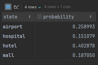

We can visualize this as a histogram:

distribution.plot(kind='bar', color='mediumorchid')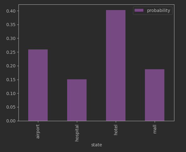

Going back to our earlier questions:

“How do you know if the data generated actually is a reasonable facsimile of the training data?” The answer revolves around deciding if our generated data has a distribution similar enough to the stationary distribution. The generated data should have a histogram roughly like what we see above.
“Are there any inputs to the process, other than the training data, that could influence whether that generated data is a reasonable facsimile?” Here the answer will be determining if the initial state or the seed or the number of steps of progress cause the generated data to not look like the stationary distribution.
“How do you know when you have enough data from a Markov Chain?” It is possible that some of the concerns of the second question above go away when enough data is generated. We will examine how much is enough for us to see approximately the correct histogram.

Lining Up The Pieces

Piece 1: “Create runs of output data. These are sequences of states.”

PyDTMC gives us a starting point for this. It takes a little tidying to map between state names and state numbers (row offsets in the adjacency matrix):

from_state_mapping =\
    {state: index_pos for index_pos, state in enumerate(adj_matrix.index)}
from_index_pos_mapping =\
    {index_pos: state for index_pos, state in enumerate(adj_matrix.index)}
simulated = model.simulate(steps=5,
                           initial_state=from_state_mapping['hotel'],
                           seed=42,
                           output_indices=True)
states = [from_index_pos_mapping[index_pos] for index_pos in simulated]

That gets us:

The result is our initial state, 'hotel', plus the 5 randomly-generated next states that we asked for.

We will build on that and create a Pandas DataFrame suited to how we will analyze generated runs.

Piece 2: “Analyze the probability distribution of the states in those runs.”

Ok, this one takes a little more coding work. We need to:

Generate the simulated run.
Treat each value in that run as a DataFrame row corresponding to a step.
Convert the string name of the step into separate column, so 'airport' is counted in a different column than 'mall'; a marker value of 1 means present, 0 means absent.
Make running aggregates at each step, so that at step 3 we have the per-state aggregate from the initial state + step 1 + step 2 + step 3.
Use those aggregates to generate the probability distribution implied at that step. This means adding the aggregates to get a total number of all states seen, then dividing the aggregates by the total.

Here we go!

# 'states' are from the simulated run above
running_df = pd.DataFrame({'state': states})
running_df.index.name = 'step'
# count how many of each state we used as of each step in the process
state_count_df = pd.get_dummies(data=running_df, 
                                prefix='', 
                                prefix_sep='').cumsum()
# add any missing states because we may not have used them all yet
# and cumsum would drop missing states from the result
model_states = adj_matrix.index.tolist()
missing_columns = set(model_states) - set(state_count_df.columns)
if missing_columns:
    for state in missing_columns:
        state_count_df[state] = 0
        # debugging is easier it we keep the state column-order canonical
        state_count_df = state_count_df[self.model_states]
# add the count aggregates to our running log
running_df = pd.concat([running_df, state_count_df], axis=1)
# turn the current row into its implied distribution
distribution_df = state_count_df.div(state_count_df.sum(axis=1), axis=0)
distributions = [row.to_frame() for _, row in distribution_df.iterrows()]
for distribution in distributions:
    # make it look like the structure of the stationary distribution
    distribution.index.name = 'state'
    distribution.rename(columns={0:'probability'}, inplace=True)
running_df['distribution'] = distributions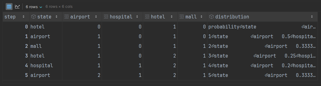

The outcome is a running total of the appearances of each state. The distribution column looks a little messy but that is because each value is itself an entire DataFrame object, which will come in handy later.

Piece 3: “Make analysis repeatable by controlling random numbers via seeds.”

We’ll be doing a decent number of runs where we want to extract the signal of what we are attempting from the surrounding noise of randomness. Because of that I decided to use random numbers generated by the Python secrets module so that I would be tapping whatever entropy backed /dev/urandom. The seeds are then saved to a Parquet file for re-use.

class SeedHandler:
    
    def __init__(self, *, num_seeds, bits_per_seed, seed_location):
        self.num_seeds = bits_per_seed
        self.bits_per_seed = bits_per_seed
        self_seed_location = seed_location

    @property
    def seeds(self):
        if not os.path.exists(self.seed_location):
            seed_values = self._make_seeds()
            self._write_seeds(seed_values=seed_values)
        else:
            seed_values = self._read_seeds()
        return seed_values

    def _make_seeds(self):
        values = []
        for i in range(self.num_seeds):
            value = secrets.randbits(self.bits_per_seed)
            values.append(value)
        return tuple(values)

    def _read_seeds(self):
        seed_df = pd.read_parquet(path=self.seed_location,
                                  engine='pyarrow')
        seed_ds = seed_df.astype(dtype=dict(seed=self.numpy_dtype))['seed']
        return tuple(seed_ds)

    def _write_seeds(self, *, seed_values):
        seed_ds = pd.Series(data=seed_values, name='seed')
        seed_df = seed_ds.to_frame()
        seed_df.to_parquet(path=self.seed_location, engine='pyarrow')

There’s more code in the Jupyter notebook, but the above shows the essence.

Piece 4: “Examine sensitivity of the runs to the choice of seed used.”

The resulting seeds will be supplied to every call of simulate(), which will be handled within the function that generates the states and builds running_df. We just need to augment that DataFrame with a 'seed' column.

for seed in seeds:
    running_df =\
        running_distributions(steps=steps,
                              initial_state=initial_state,
                              seed=seed)
        # get a 'step' column from the existing index
        running_df.reset_index(drop=False, inplace=True)
        # and add the seed
        running_df['seed'] = seed

That gets us two out of three pieces of what will become our multi-index.

Piece 5: “Use all the possible initial states as initial states.”

And now we get our third piece of the multi-index. We need another loop around the code above so we can supply different choices of initial_state, add a column to track it, build an index from the three parts, and pd.concat() the running_df from each (initial_state, seed) combination.

index_columns = ['initial_state', 'step', 'seed']
across_states_and_seeds_df = None
for initial_state in model_states:
    for seed in seeds:
        running_df =\
            running_distributions(steps=steps,
                                  initial_state=initial_state,
                                  seed=seed)
            running_df.reset_index(drop=False, inplace=True)
            running_df['initial_state'] = initial_state
            running_df['seed'] = seed
            # create the multi-index
            running_df.set_index(index_columns, drop=True, inplace=True)
            if across_states_and_seeds_df is None:
                across_states_and_seeds_df = running_df
            else:
                across_states_and_seeds_df =\
                    pd.concat([across_states_and_seeds_df, running_df],
                              axis=0)

Piece 6: “Assess how long it takes the model to forget the state it started with.”

This will be examined in two different ways.

Analytically.
From the data.

The analytical part is supplied by a PyDTMC model property:

model.mixing_rate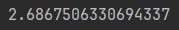

I believe this property is misnamed. The implementation appears to be what is usually called the “relaxation rate” or “convergence rate”. This is the rate at which deviations from the stationary distribution shrink as more steps are added to the chain generated. It’s derived from the same eigenvalue information as the spectral gap.

To get an estimate of how many steps that implies — the mixing time — before a desired amount of convergence is achieved, we would have to adjust for how close we want the generated distribution to be to the stationary one.

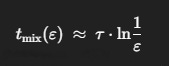
This is a bit opaque since we aren’t really indicating what we are measuring via that rate, but as a first approximation we’ll use epsilon=0.001:

epsilon = 0.001
taxi_structure.model.mixing_rate * math.log(1 / epsilon)

That’s our analytical reference point, we want to see how the chain distributions look when we have the 19th step after the initial state.

The reason I picked an epsilon that small is because we haven’t discussed what kind of distance should matter. I did some digging via the PyDTMC source code, Wikipedia, and several Monte Carlo texts to get an answer.

If I were to use the PyDTMC mixing_time() method I believe it uses the square root of the dot product between the stationary distribution and the distribution of the generated chain.
The more usual mathematical definition is based on the greatest absolute difference between the two distributions, called the “Total Variation Distance” (TVD). It’s definitely the one I find discussed in material on convergence.

The second is closer to what we want, but not quite. We care about:

Average closeness: what PyDTMC provides.
Worst-case closeness: what TVD provides.
Similarity of shape between the two distributions: which neither provide.

We want all three, and getting the third with a small value gets you the first two.

As a reminder of what we’re trying to achieve in this piece, we want to know when the choice of initial state no longer has a meaningful bias on the distribution of the chain. By comparing the distribution of the generated chain to the stationary distribution, when they are similar enough we are declaring that there is no longer any level of bias from the initial state that we would care about.

For this reason I added a different measure of closeness to the code, based upon the Jensen-Shannon Distance (JSD). It is histogram-friendly by being symmetric (comparing A to B is the same as comparing B to A), and robust to empty bins:

eps: float = 1e-9
adjusted_sample = (sample + eps) / (sample + eps).sum()
distance = sp_sd.jensenshannon(p=stationary_distribution,
                               q=adjusted_sample)[0]

The adjustment shown deals with a limitation in JSD when the two distributions get very close and you’re faced with the limit of dividing a small value by another value that is approaching zero.

There is a bit more code to getting the distance behaving when faced with numerical error, which is in the Jupyter notebook. It’s a little bit of a hack but the alternative would be to implement JSD from scratch to deal with a special case where numerical error triggered sqrt(negative number) instead of sqrt(zero). I found in practice a small number of random seeds tripped over that case when generating large sequences.

Assembling the Pieces

Now that we have a notion of distance, we need to add it to our computation of the running results.

We will want to examine that distance at each step and see if it is mostly declining, and what our measure is at the 19th step we derived analytically.

# 'states' are from the simulated run above
running_df = pd.DataFrame({'state': states})
running_df.index.name = 'step'
# count how many of each state we used as of each step in the process
state_count_df = pd.get_dummies(data=running_df, 
                                prefix='', 
                                prefix_sep='').cumsum()
# add any missing states because we may not have used them all yet
# and cumsum would drop missing states from the result
model_states = adj_matrix.index.tolist()
missing_columns = set(model_states) - set(state_count_df.columns)
if missing_columns:
    for state in missing_columns:
        state_count_df[state] = 0
        # debugging is easier it we keep the state column-order canonical
        state_count_df = state_count_df[self.model_states]
# add the count aggregates to our running log
running_df = pd.concat([running_df, state_count_df], axis=1)
# turn the current row into its implied distribution
distribution_df = state_count_df.div(state_count_df.sum(axis=1), axis=0)
distributions = [row.to_frame() for _, row in distribution_df.iterrows()]

# ---> changes for distance are below
distances = []
for distribution in distributions:
    # make it look like the structure of the stationary distribution
    distribution.index.name = 'state'
    distribution.rename(columns={0:'probability'}, inplace=True)
    distance = distance_from_stationary(sample=distribution)
    distances.append(distance)
running_df['distance'] = distances
running_df['distribution'] = distributions

Now we will have that distance and its corresponding distribution available to us for visual comparison to the stationary distribution.

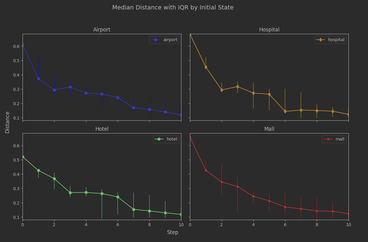
First, let’s look at a run with 200 seeds and 10 steps. We’ll keep the number of steps small this time in order to make it easier to examine details of the image.

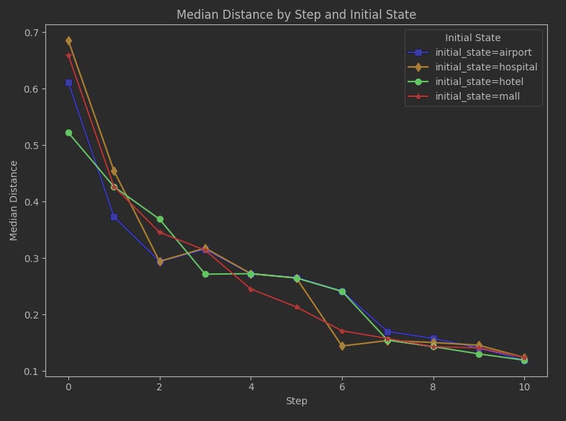
Notice how at at the start (step 0), where all we have is the initial state, the two initial states that are closest to the stationary distribution are 'hotel' then 'airport'. This makes sense, as these are also the two states with the highest probabilities in the stationary distribution; 'hotel' is the highest probability and by distance measure it is the closest. At least JSD as the distance measure isn’t showing something entirely off-base right from the start.

As the run progresses, the median outcomes for each initial state converge, and by step 7 we’re seeing they don’t differ much from each other. The rest of the run going forward won’t likely be about specific initial states, but just the overall challenge of any state to result in data that closely approximates the stationary distribution.

Unfortunately we may be jumping the gun a bit at 7. Let’s look at seed sensitivity. We can plot the interquartile ranges on each step after the initial state:

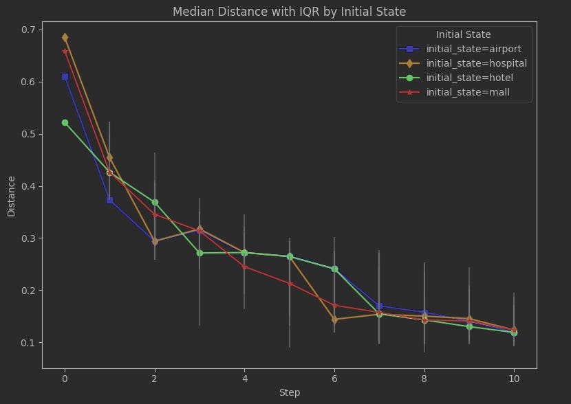
The per-seed results are still jumping around quite a bit. This isn’t hugely surprising. The number of states is effectively a sample size, and when the sample size is something like 7 then it doesn’t take much to perturb the range of distances produced.

We can get an ever better look at this with initial states in separate plots.

So not only are the results variable per seed, the variability varies by initial_state. Clearly 7 steps is too soon to declare we’ve moved beyond bias.

We had our analytic estimate of 19 steps. Let’s take the analysis out to 30 steps so we can see 19 in a broader context.

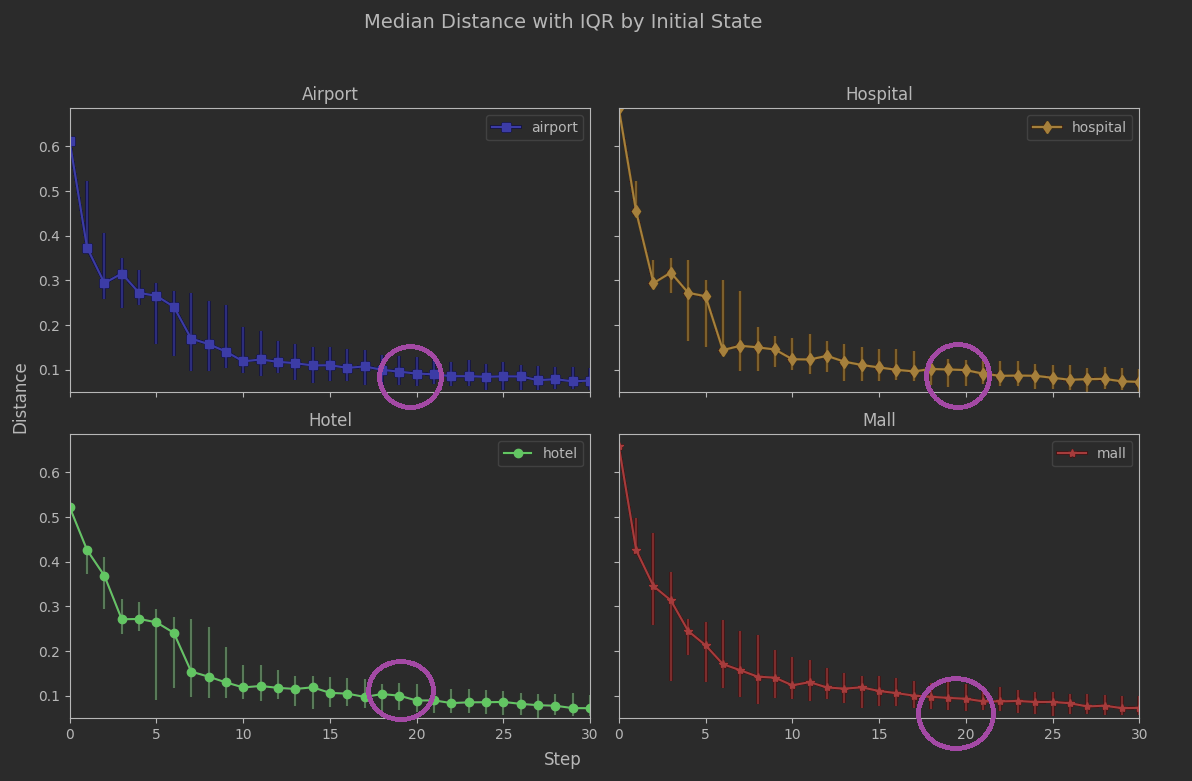
The region around 19 steps looks quite stable. The variability is low, and low across all initial_state values. The rate of convergence is slowing down a lot, but that’s probably not a surprise. As a reminder from the previous article, the spectral gap being closer to 0 than 1 suggested convergence could be sluggish:

model.spectral_gap

Time to take a look at the actual histograms at step 19 and see what they tell us.

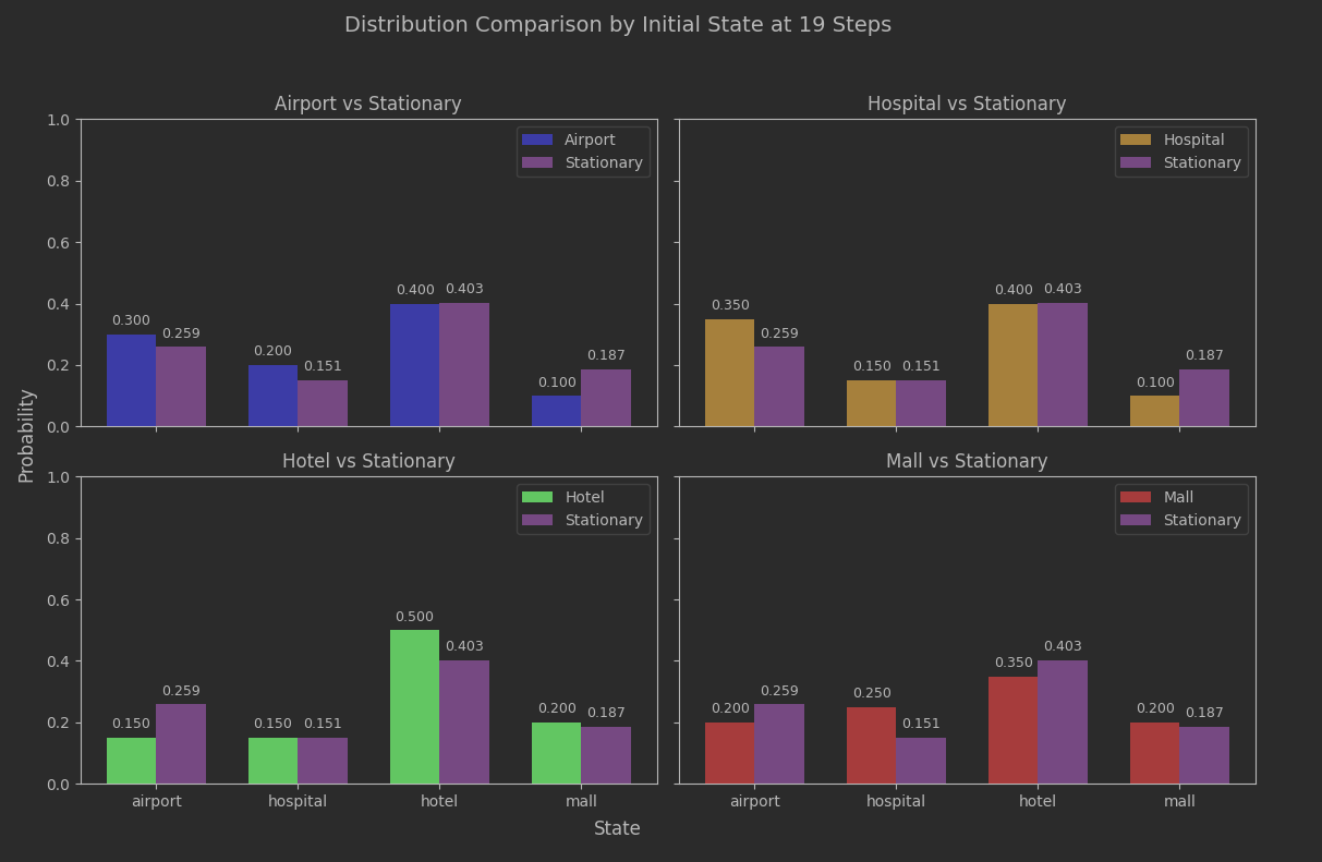
Not too bad. The estimated convergence seems to have relevance. Since this batch of data went out to 30 steps, we can compare to that.

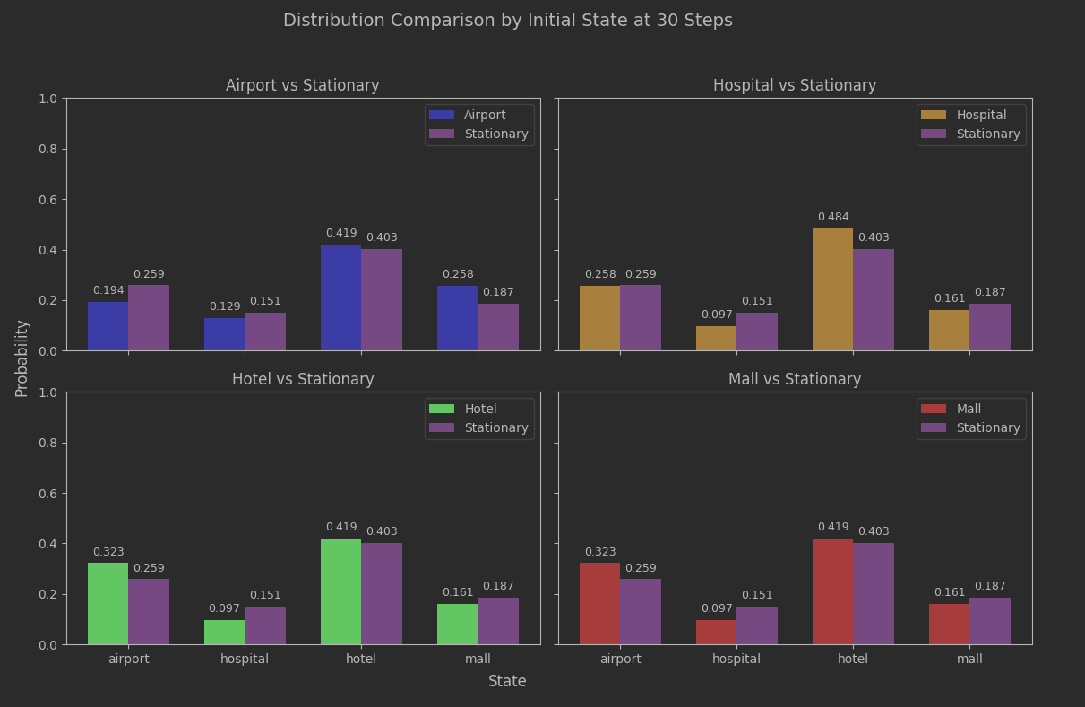
Slightly better, but not game-changing. The important thing is that we aren’t seeing any meaningful bias based on what the initial state was, and as earlier plots showed the IQR variance based on the seed choice was narrowing as well.

Summary

We wanted to generate data with this model and have a reasonable expectation that the data looked similar to what it was trained on. That is workable at 19 steps and would get progressively better over time.
There would be no real need to worry about a better or worse choice of initial state or using data generated across multiple seeds, neither initial-state bias nor seed variance are problematic for chains at least 19 steps long.
Our use of the Jensen-Shannon Distance appears safe. This isn’t really enough material to critique it versus other distance measures, but that wasn’t the goal. What we wanted was reasonably-similar histogram structure, which is what we have.
The estimate of a mixing time (number of steps until viable convergence) lined up with the empirical results, which actually was a nice surprise. Going into the analysis I was skeptical that we would see decent histogram shape that early in the sequence.

References

Jupyter notebook for this article.
NetworkX API reference.
Pandas API reference.
PyDTMC PyPi.
Häggström, Olle, “Stationary distributions,” in Finite Markov Chains and Algorithmic Applications. London Mathematical Society Student Texts, vol. 52, Cambridge University Press, 2002, pp. 28-38.
Brémaud, Pierre, “Convergence Rates,” in Markov Chains: Gibbs Fields, Monte Carlo Simulation and Queues, Texts in Applied Mathematics, vol. 31, Springer Cham, 2020, pp. 289–329.
“Total variation distance of probability measures,” in Wikipedia, accessed 2025-08-28, permanent link (revision) <https://en.wikipedia.org/w/index.php?title=Total_variation_distance_of_probability_measures&oldid=123456789>.
“Markov chain mixing time,” in Wikipedia, accessed 2025-08-28, permanent link (revision) <https://en.wikipedia.org/w/index.php?title=Markov_chain_mixing_time&oldid=1233574639>.